
Part 03
Areas
Saved boundaries, and the four things you can do with one.
Every boundary you save becomes an area, and an area is the unit almost everything else hangs off. Analyses, trends, composites, comparisons and monitors are all scoped to one.
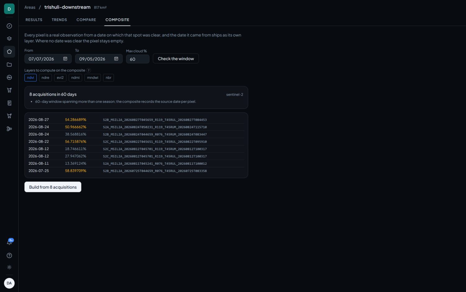
The Areas table
Areas
One row per boundary: name, project, the satellite it was last searched against, its size in km², who created it and when. Search areas filters by name. Draw area and Upload boundary both jump to Explore with the right tool armed.
The Analyse link on each row is the shortest path from a saved boundary to a new run, and opens the dialog covered in part five. The cross removes the area. Removing an area does not remove the results already produced from it.
Inside an area
Areas › any area
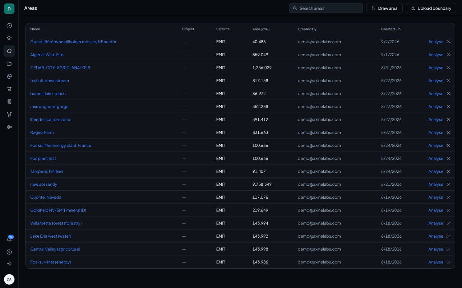
Opening an area gives four tabs.
| Tab | What it shows |
|---|---|
| Results | Every analysis run over this area, newest first. |
| Trends | One statistic of one layer, plotted through time. |
| Composite | A cloud-free picture of the area assembled from several dates. |
| Compare | The change screen from part seven, pinned to this area. |
Trends
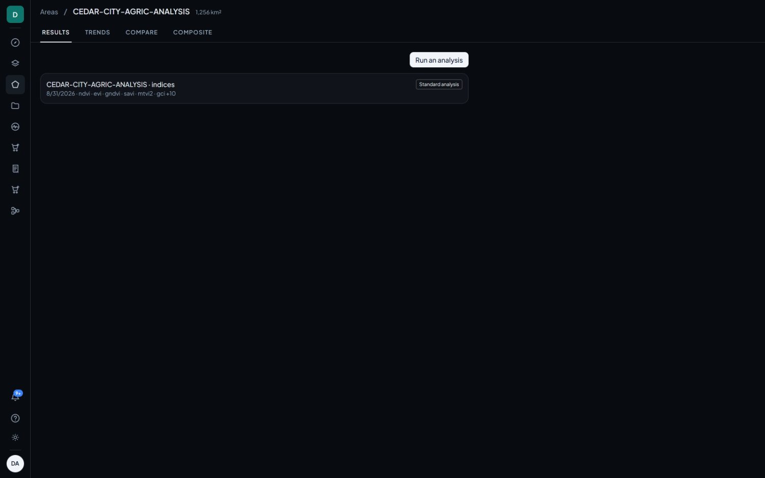
Choose a satellite, a layer and a statistic, then select Plot. The tab charts that statistic across every analysis of this area, in order. It is the fastest way to see whether today's reading is unusual or ordinary.
Three statistics are available.
| Statistic | Meaning |
|---|---|
| Area mean | The average across the mapped area. |
| 90th percentile | The value nine tenths of the mapped area falls below. |
| Share of area above a value | The fraction of the mapped area exceeding a per-pixel value you supply. |
Two rules change how the line should be read, and both stay visible.
- A series belongs to one sensor. Sentinel-2 and Landsat do not read the same number over the same ground, so mixing them into one line would manufacture steps that are instrument changes rather than events.
- Scenes that could not be measured are listed, not dropped. Each is named with the reason. A gap in the chart should look like a gap in the evidence, rather than like a period in which nothing happened.
A trajectory needs at least two analyses over the area on the same sensor. If there is only one, the tab says so and lists the single reading rather than drawing a line through one point.
Composite
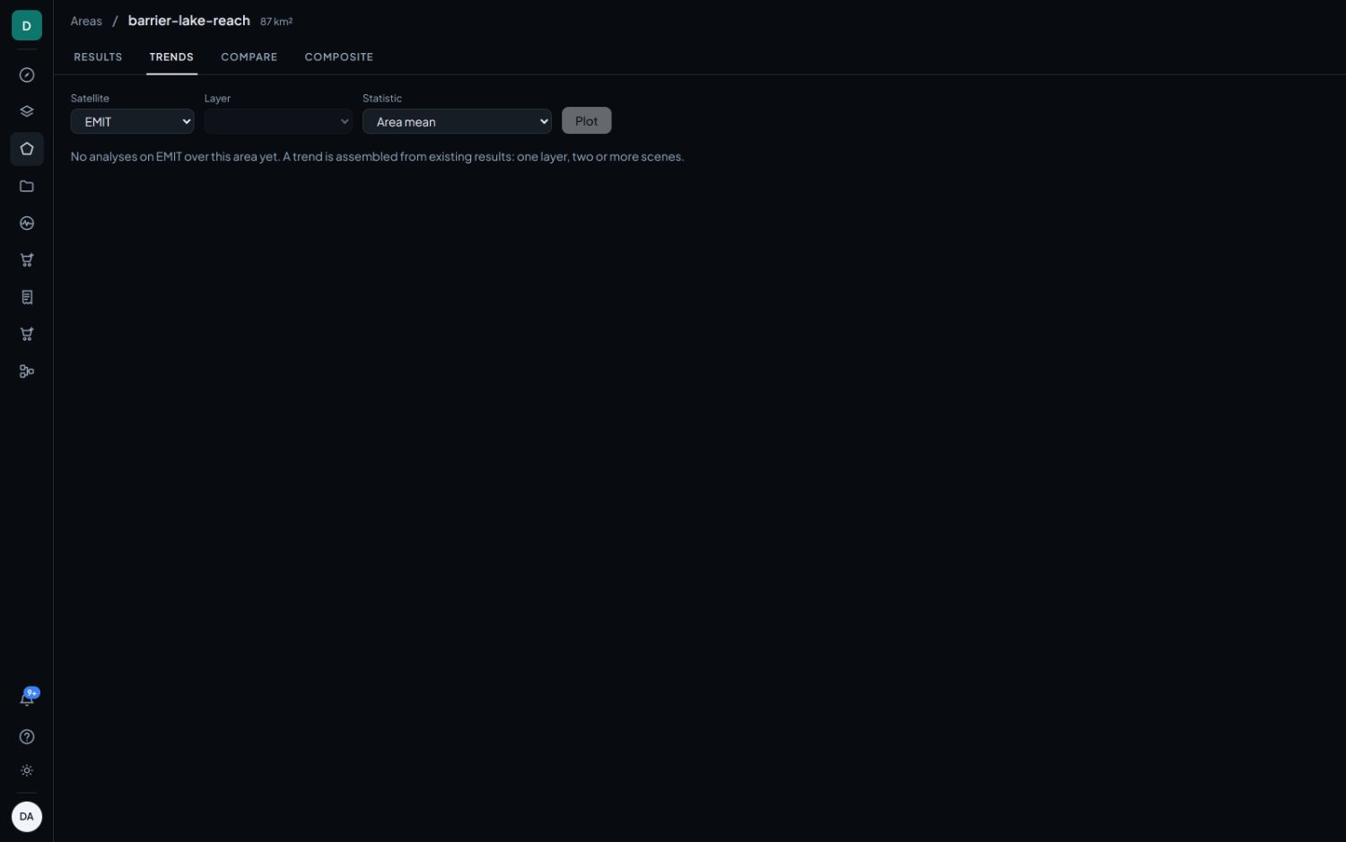
A cloud-free image of the area assembled from several dates inside a window you choose. Useful when no single acquisition is clear enough to work with.
Set From, To and Max cloud %, then select Check the window to see which scenes qualify before anything is computed. Choose the layers to compute on the composite, and build it.
Nothing is reconstructed and nothing is predicted. Each pixel is taken from
a date on which that pixel was genuinely clear, or it is left empty. The
date each pixel came from is published as its own layer,
_SOURCE_DAY, alongside how many observations went into it,
_OBS_COUNT, and how far apart they were,
_DATE_SPREAD. Read those before treating a composite as a
snapshot, because no pixel of it was seen on any single date in the way the
picture implies.