Part 05

Running an analysis

One dialog takes you from a saved boundary to a queued job.

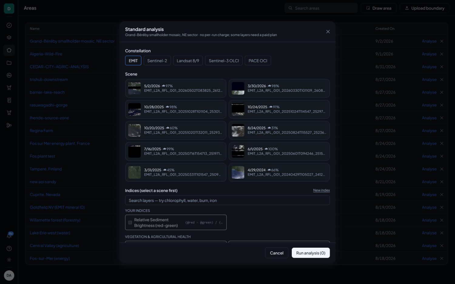
Reach the dialog from Analyse on any area row, from an area's own page, or by carrying a selection over from the analytics catalogue. It asks for three things in order: a constellation, a scene, and the layers to compute.

Constellation and scene

Pick the constellation first. It decides which scenes are searched and which layers are offered. The scene grid shows what covers the area, newest first, each with its acquisition date, cloud percentage, quicklook and full granule identifier. A selected scene is marked three ways, with a ring, a tint and a tick, so the selection cannot be lost to a rendering accident.

Read the cloud figure together with the quicklook rather than instead of it. Cloud percentage is measured over the whole granule, and a scene reported at 60 per cent can be perfectly clear over a small area inside it.

Choosing layers

Layers are grouped the way the catalogue groups them. The search box takes a name or the thing you are looking for, such as chlorophyll, water, burn or iron, and shows a hit count. Two behaviours are worth knowing.

• Layers you have already selected but which the current search hides are still counted in the run, and the dialog says so with a Show all link. A filter never silently drops a selection.
• Esc clears the search box rather than closing the dialog. Losing a half-built selection to a keystroke meant for the search box is not a recoverable mistake.

A layer the chosen source cannot carry is greyed out, with the source's own reason on hover rather than a guess. A layer that runs but is not separable at this band width carries a screening chip beside its name.

When layers are dropped

If you carried a selection in from the catalogue and then chose a scene that cannot support part of it, an amber block lists exactly which layers were dropped and why, before you run anything. It does not tell you to pick a different constellation, because a dropped layer is not guaranteed to run on any other one. A workspace formula built on EMIT wavelengths runs nowhere else. Each row carries its own reason instead.

Building your own index

Standard analysis › New index

New index opens a builder for a formula the catalogue does not carry. Choose a mode, such as normalised difference or a plain ratio, then the bands. Wavelength bands are shown in nanometres rather than as internal keys, because a wavelength is what you are actually choosing. Pick a colour ramp and save it.

A saved index appears under Your indices at the top of the layer list in every future run, with its expression printed beside it. It is scoped to the workspace, so colleagues get it too. An index built on wavelengths that one sensor has and another does not is greyed out on the sensor that lacks them.

The two standing lanes

Below the index list sit two products that are not indices. Each is ordered on its own button and returns as a normal result.

Evapotranspiration screening

An SSEBop surface energy balance over the Landsat thermal band. One order computes both the actual ET layer and the ET fraction. It covers the conterminous United States for now. An area outside that is refused at order time with the reason, rather than returning a number that means nothing.

Canopy biophysics screening

A physical-model inversion over Sentinel-2's red edge, returning leaf area index, canopy chlorophyll and the retrieval spread for each, as one result. Bare soil and water return no value, with the reason attached. Leaf area index saturates above 5, and the spread layer shows where that is happening.

Running, and what happens next

Run analysis carries the count of layers that will actually run. The button stays inert until a scene is chosen and at least one layer is selected.

A plan refusal appears in the footer naming the blocked layers and the plan that unlocks them, with a link to Plans. Nothing partial is run and no order is created.

Otherwise the job is queued and you can close the dialog. It moves through named stages, from fetching the scene to computing to publishing, and a notification arrives when it finishes. The result appears in Results and on the area's own Results tab.