Part 06

Reading a result

The densest screen in the studio, and the one worth learning properly.

It is the same screen for every product. What changes is which panels mount and how they are arranged, and the studio decides both from the layers the result actually carries.

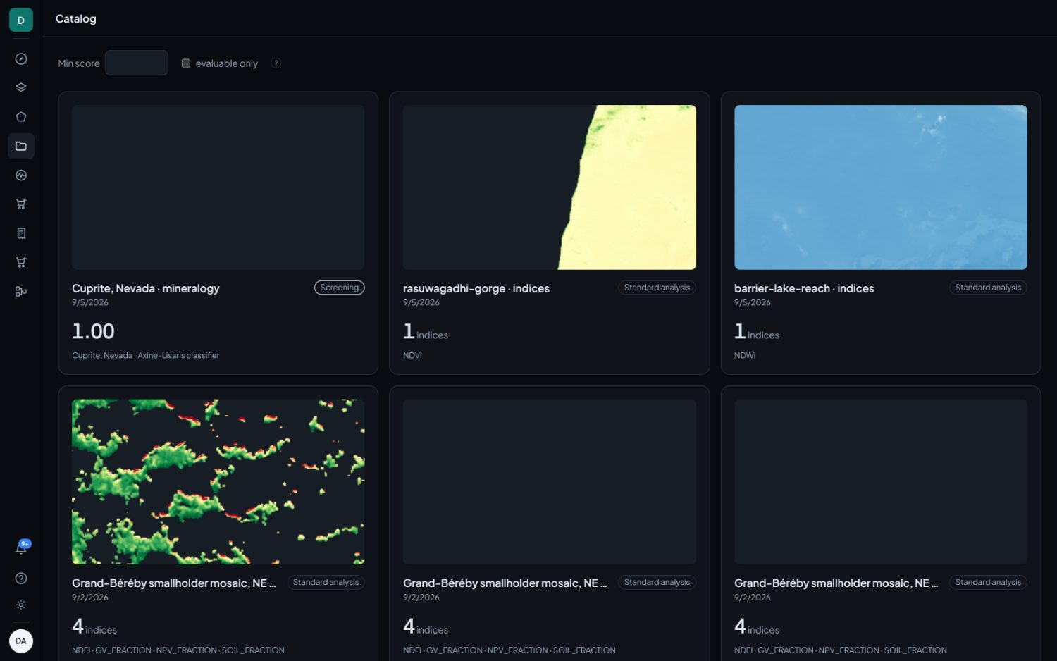
The Catalog list

Results

One card per finished analysis, newest first. The date on a card is when the satellite saw the ground, not when we processed it. The badge on the right is the validation posture. A result that produced a score shows it in place of the layer count.

One filter sits above the grid.

Evaluable only hides results the studio declined to summarise, usually because too much of the area was cloud, water or low signal. Those results are still real and still mapped. What is missing is a summary statistic, not the pixels.

The Catalog grid. Thumbnails are the result's own render, so a card is recognisable before you read its title.

Anatomy of the screen

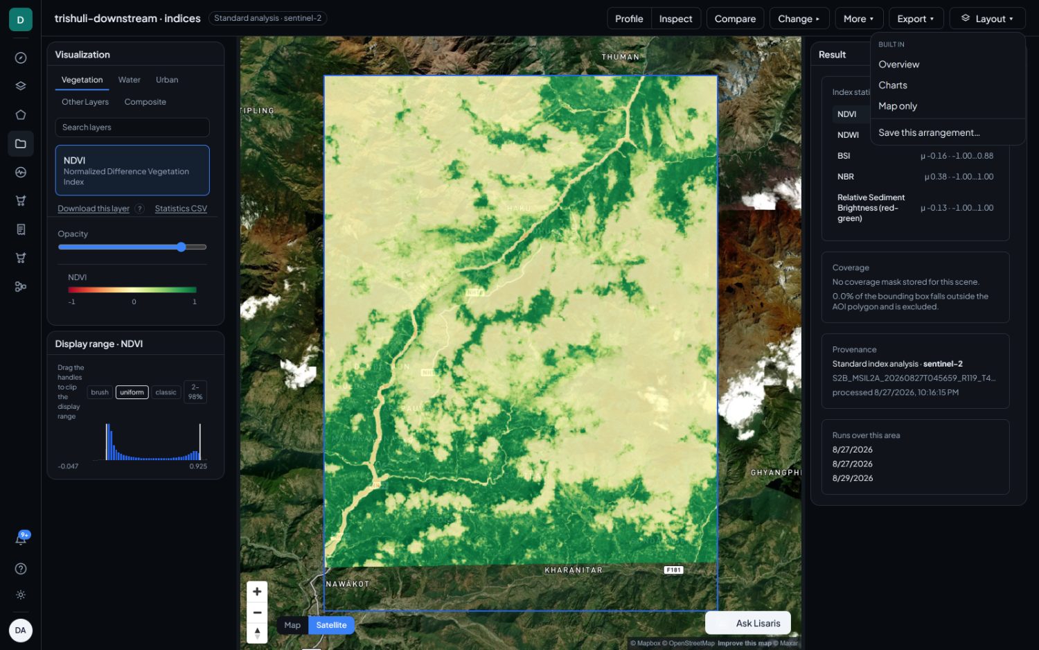
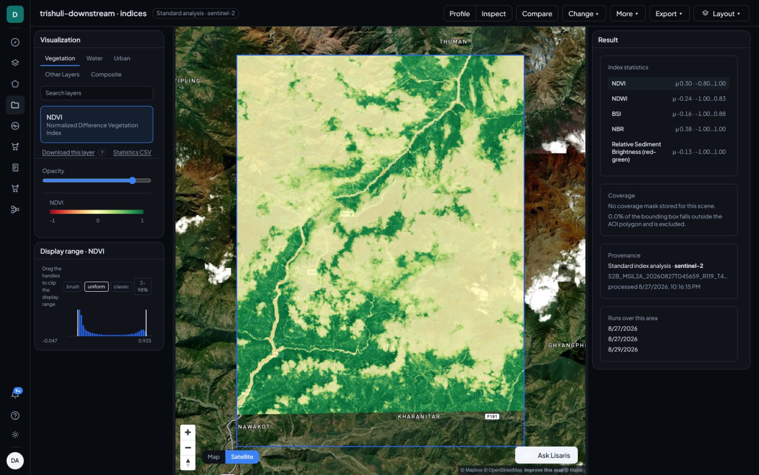
Five regions, in the default arrangement.

Region	Holds
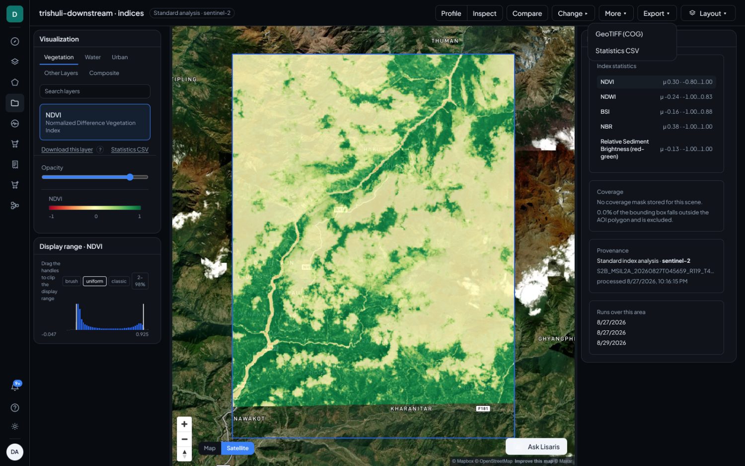
Title bar	The result name, its posture badge, the map tools, and the Compare, Change, More, Export and Layout menus.
Left dock	Visualization, with Display range beneath it. What the map is showing.
Map	The raster over a basemap, with the scene-quality chip floating above it.
Right dock	Result, and Materials where a library fit ran. What the result is worth.
Bottom dock	The charts: Spectral graph, Profile and Detection confidence.

Visualization

The layer catalogue for this result. Layers are grouped into tabs by what they measure, so a canopy pack opens on Vegetation, Water, Urban, Other Layers and Composite. A search box filters across all of them, which matters on a result carrying twenty-six layers.

Beneath the layer list:

Opacity for the active layer over the basemap.
Smooth view, on classified results, swaps the raw classification for its smoothed version. It is a display choice and the statistics do not change.
Download this layer gives you that layer as a cloud-optimised GeoTIFF, georeferenced and ready for a GIS.
Statistics CSV gives you the numbers behind the panel on the right.
The legend for the active layer. A classified layer gets one swatch per class. A continuous layer gets a colour bar with the range and the unit it covers. No-data is drawn as a hatch and never as a colour, so it cannot be mistaken for a value.

Display range

A histogram of the active layer with two draggable handles. Everything below the left handle draws as the bottom of the ramp, and everything above the right handle draws as the top. This is the control that pulls detail out of a narrow band of values, and it is the operative act on any thresholded read.

Drag the handles to clip the display range.
brush lets you drag across the histogram to highlight a band of values on the map without changing the ramp.
uniform and classic switch between a perceptually uniform ramp and a classic rainbow. Uniform is the default and the honest one, because equal steps in value are equal steps in apparent colour. Rainbow is offered because some conventions expect it.
2 to 98% resets the handles to the second and ninety-eighth percentiles, which is the usual starting point.

Display only

Clipping changes what is drawn and nothing else. The measured values, the statistics in the Result panel, the CSV and the GeoTIFF are all untouched. You can mislead yourself into a different picture with this control, but not into a different number.

The Result panel

The right-hand rail. Its blocks, from the top.

Score, where a product produces one

Shown with its posture badge and an explanation of what that badge licenses. A screening score is for shortlisting ground, not for reporting. Where the model works best expands to the conditions under which the figure means the most.

Statistics

Per layer: the mean, and the first to ninety-ninth percentile range. These cover measured ground only, never the whole box.

Composition, on a classified result

The area fraction of each class, with a bar, and the masked fraction listed separately underneath so the fractions visibly do not include it.

Coverage

What was masked and why, and how much of the bounding box fell outside your polygon and was excluded. Read this before any percentage above it.

One line to check every time

If Coverage says Statistics cover the bounding box around your boundary, the percentages above it were computed over the rectangle that encloses your polygon rather than over the polygon. On a drawn rectangle the two are the same. On an uploaded boundary they are not, and on a corridor the rectangle can be many times larger than the ground you selected.

The map and the layers are unaffected. Re-running the analysis recomputes the summary against the polygon.

Provenance

The engine that ran, its version, the exact granule identifier and the processing timestamp. This is the block to quote when somebody asks where a number came from, and the block to check when two results disagree.

Runs over this area

Every earlier pass over the same ground, with its score where it had one. Worth reading before you act on today's number. If a score moved sharply between two runs a day apart, the thing that changed is far more likely to be the engine version than the ground, and Provenance will tell you.

Scene quality

The chip floating over the map states what fraction of the ground was measurable. It has three levels, and the level decides how loudly it speaks.

Exposure	Shown as	Meaning
50% and above	Quiet chip	A good scene. Stated once, collapsed, so it does not shout.
10% to 50%	Amber strip	Limited, and persistent, because the denominator changes what the statistics mean.
Below 10%	Red strip	Unusable, and not dismissible. The result stays viewable, because you may legitimately want the half a per cent that was seen, but absence of detections here means nothing.

Known instrument artefacts ride alongside as their own chips, so a sensor-specific quirk is named rather than left to look like ground.

The four map tools

A segmented control in the title bar. They are mutually exclusive, so picking one drops the other. Which of them appear depends on what the result carries.

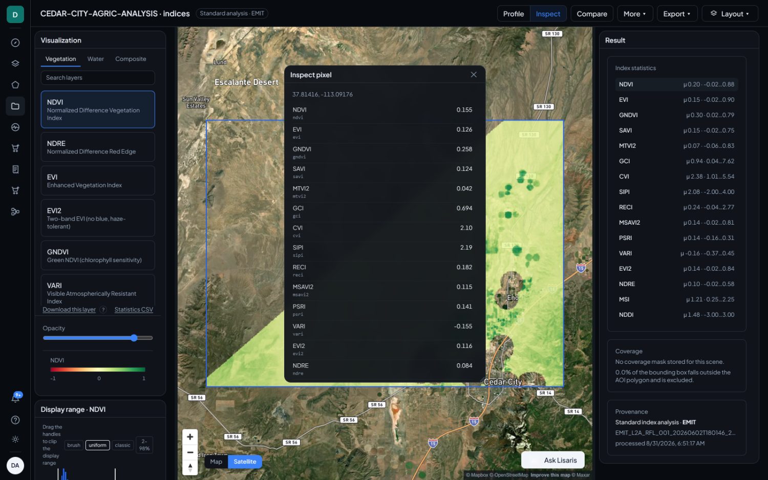
Inspect

Click any pixel and read every layer's value there, with each layer's unit where it has one. This is the only honest way to read a stack whose layers mean different things, because a detection score, its sensitivity and its false-positive risk are meaningless apart.

Values are printed at a precision that matches their magnitude, so a genuine trace of 0.00028 does not print as 0.000 beside a four-figure number.

Inspect on a sixteen-layer canopy result. One click returns every index at that coordinate, with the scene-wide statistics for the same layers on the right.

Profile

Draw a line on the map and the bottom dock charts every layer's value along it, against distance in kilometres. Continuous layers draw as lines, and a classified layer draws as bands in its own class colours. This is the tool for reading a gradient, whether downslope, across strike or along a watercourse.

Spectral

Available only on results that carry full spectra, which in practice means EMIT. Pick two pixels and the graph charts their reflectance against wavelength side by side, with continuum removal available and the diagnostic absorption windows tinted. Reference spectra from the spectral library can be overlaid, deliberately drawn dimmer than the measured curves, because they are context for the pixel rather than competing readings.

Minerals

Available only where a library fit ran. Click a pixel and it lists every material identified there, with its fit.

The Materials browser

Where a library fit ran, the right dock carries a browser of every identification in the scene, by mineral family. There are two display modes.

Dominant map shows one material per pixel, the one that fitted best.
Overlays draws up to four materials together as translucent ramps, for comparing distributions.

Four is a budget rather than an arbitrary cap. Beyond about four translucent ramps on one basemap the classes stop being tellable apart. Two materials from the same family would render identically, because a ramp is a family hue, so the second is given a separate slot hue and the legend names the substitution rather than letting you read one map as the other.

Fit	Shown as	Reading
0.70 and above	strong	A confident identification.
0.50 to 0.70	ok	Usable, and worth corroborating.
Below 0.50	weak	Below the reporting floor. Shown, not counted.

A material occupying fewer than thirty pixels is not offered as a distribution. At that size the shape on the map is noise, whatever the fit says.

Compare, More and Export

Compare

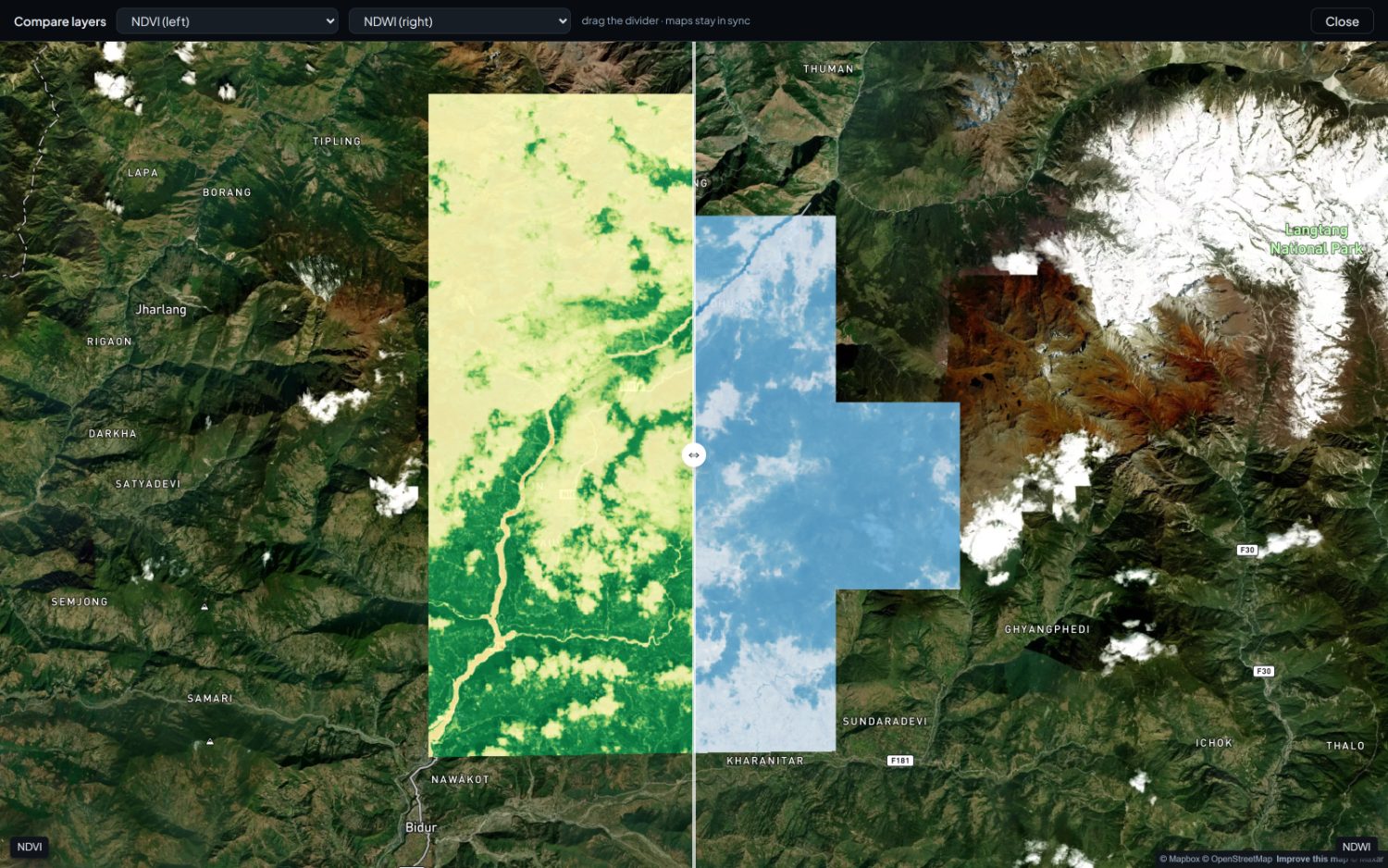
Two layers of the same result, side by side under a draggable divider, with the two maps sharing one camera. Use it to check whether two indices agree about the same ground. Comparing two dates is a different action, covered in part seven.

The occasional actions, each carrying a tick when it is on.

Detection chart, on library-fit results, charts band depth against fit quality for each detection window. It is how marginal detections become visible as a cloud rather than as a number.
Dim weak fits veils the map wherever the fit is weak, so a strong pattern is not read across ground that barely fitted anything.
Publish to client, for admins and owners. See part eleven.

Export

What is offered depends on what the result is.

Export	Available on
GeoTIFF (COG)	Every result.
Statistics CSV	Every index result.
Features GeoJSON	Results that produced vectors. On a plume product this is the plume outlines with their integrated mass and emission rate.
Clusters GeoJSON	Classified results.
Score table CSV	Classified results.
Summary PDF	Classified results. Carries the limits text expanded.

The Export menu. Raster and statistics come off any analysis, and the vector and document products appear where the result carries them.

Layouts, per product

The built-in arrangements offered in the Layout menu are chosen for what the result is, because the reading act differs. A mineralogy arrangement is not offered on a canopy result or the reverse, since applying one there would produce a rail of panels that cannot mount.

Result	Leading layout	Why it is cut that way
Mineralogy	Mineralogy review	The widest right rail of any layout, because the Materials browser is the longest panel in the product and it is read against the score directly above it.
Mineral indices	Mineral indices	Agreement between several band depths, read at a pixel and along a path.
Vegetation	Vegetation review	Twelve to twenty-six continuous layers read as patterns within one scene, so the layer list takes the widest left rail and the transect gets the bottom to itself. Inspect docks right, so a click reads every index beside the statistics.
Water	Water review	Water-quality retrievals are read by threshold, which is the histogram brush, and a brush needs width. Display range therefore moves to the bottom dock.
Plume	Plume review	Inspect is docked at the top of the right rail rather than floating, because an enhancement means nothing without the sensitivity and the confuser value at the same pixel.
Drainage and seep	Drainage review, Seep review	One shape under two names: agreement between several layers at a pixel and along a path downslope.
Composite	Composite quality	The only question a composite raises is which pixels to trust, answered by the observation-count and source-date layers. There is no bottom dock at all, so a date seam stays visible at scale.

Overview, Charts and Map only are offered everywhere.